The H Score
The Key Points
H-score is our first step in introducing neural-network-based methods to compute modal decomposition from data. It is a loss metric used in the training of neural networks in a specific configuration, which we call the “H-Score Network.” The result is approximately equivalent to a conventional end-to-end neural network with cross-entropy loss, with the additional benefit of allowing direct control of the chosen feature functions. This is an important conceptual step to turn the goal of learning from learning a probability model to learning feature functions. In practice, H-score networks have a number of natural extensions that allow more flexible operations to incorporate external knowledge.
The H-score Network
Low-Rank Approximation of Probabilistic Models
The motivation of modal decomposition is to find the rank-\(k\) approximation
\[\begin{equation} \{(\sigma_i^\ast, f^\ast_i, g^\ast_i), i=1, \ldots, k\} =\arg\min_{\substack{(\sigma_i \in \mathbb{R}, f_i \in \mathcal {F_X}, g_i \in \mathcal {F_Y}),\\ i=1, \ldots, k}} \; \left\Vert \mathrm{PMI}- \sigma_i\cdot \left(\sum_{i=1}^k f_i \otimes g_i\right)\right\Vert^2 \end{equation}\]The Constraints: The above problem is slightly different from our original definition of modal decomposition, where we had a sequential way to find the \(k\) modes. This sequential procedure solves the optimization problem (1). It also ensures the solution to satisfy a number of constraints:
- the feature functions all have zero mean and unit variance;
- the scaling factor of the \(i^{th}\) mode, $\sigma_i$, is separated from the normalized features;
- the feature functions are orthogonal: \(\mathbb E[f^\ast_i f^\ast_j] = \mathbb E[g^\ast_i g^\ast_j] = \delta_{ij}\),
- there is a descending order in \(\sigma_i\), the correlation between \(f^\ast_i\) and \(g^\ast_i\).
We refer to the optimal choice of \(\{(\sigma^\ast_i, f^\ast_i g^\ast_i), i = 1, 2, \ldots,k\}\) that satisfies these constraints, or obtained with the sequential procedure, as the modes of the given dependence model.
One can also run an optimization (1) without any of these constraints. The result is also a set of feature function pairs, one of many equally good low-rank approximations to the PMI function, which can be obtained as linear combinations of the ordered orthonormal feature functions in modal decomposition.
It turns out that this later unordered low-rank approximation is more closely related to the operation of commonly used neural networks, which will be discussed later in this page.
H-Score: the Definition
In this section, we ignore the constraints in modal decomposition and work only on the objective function. For convenience, we introduce a vector notation: we write column vectors \(\underline{f} = [f_1(\mathsf x), \ldots, f_k(\mathsf x)]^T\), \(\underline{g} = [g_1(\mathsf y), \ldots, g_k(\mathsf y)]^T\). Since we do not restrict the feature functions to be normalized, we do not need the scaling factors $\sigma_i$’s. Now, we use a short-hand notation.
\[\sum_{i=1}^k f_i(x)\cdot g_i(y) = \underline{f} \otimes \underline{g}\]and the optimization (1) becomes a simple form:
\[\underline{f}^\ast, \underline{g}^\ast = \arg\min_{\substack{\underline{f} \in \mathcal{F_X}^k\\ \underline{g} \in \mathcal{F_Y}^k}} \; \left\Vert \mathrm{PMI} - \underline{f} \otimes \underline{g}\right\Vert^2\]This objective function is still not easy to use since to evaluate it, we need to know \(\mathrm{PMI}\), which is equivalent to the probability model \(P_{\mathsf{XY}}\) we need to learn. The following is a nice trick: for a given model \(\mathrm{PMI}\), the above optimization is equivalent to
\[\underline{f}^\ast, \underline{g}^\ast = \arg\max_{\substack{\underline{f} \in \mathcal{F_X}^k\\ \underline{g} \in \mathcal{F_Y}^k}} \; \left\Vert \mathrm{PMI}\right \Vert^2 - \left\Vert \mathrm{PMI} - \underline{f} \otimes \underline{g}\right\Vert^2\]Now, with a few steps of algebra hidden below, it is not hard to check that this objective function can be approximated in a computable form
Consider the above objective function:
\[\begin{align} &\left\Vert \mathrm{PMI}\right \Vert^2 - \left\Vert \mathrm{PMI} - \underline{f} \otimes \underline{g}\right\Vert^2\nonumber\\ &= 2 \left\langle {\mathrm{PMI}}, \underline{f} \otimes \underline{g} \right\rangle - \left\Vert \underline{f} \otimes \underline{g} \right\Vert^2\nonumber\\ &= 2 \sum_{x,y} P_{\mathsf x}(x) P_{\mathsf y}(y) \cdot \mathrm{PMI}(x,y) \cdot \left(\sum_{i=1}^k f_i (x) g_i(y) \right) \nonumber\\ & \qquad -\sum_{xy} P_{\mathsf x}(x) P_{\mathsf y}(y) \cdot \left(\sum_{i=1}^k f_i (x) g_i(y)\right)^2\\ &\approx 2 \sum_{x,y} P_{\mathsf x}(x) P_{\mathsf y}(y) \cdot \left(\frac{P_{\mathsf{xy}}(x,y) - P_{\mathsf{x}}(x)P_{\mathsf{y}}(y)}{P_{\mathsf{x}}(x)P_{\mathsf{y}}(y)}\right) \cdot \left(\sum_{i=1}^k f_i (x) g_i(y) \right) \nonumber\\ & \qquad -\sum_{xy} P_{\mathsf x}(x) P_{\mathsf y}(y) \cdot \left(\sum_{i=1}^k f_i (x) g_i(y)\right)^2\\ &= 2 \sum_{i=1}^k \left(\mathbb E_{\mathsf {x,y} \sim P_{\mathsf {xy}}}\left[ f_i(\mathsf x) g_i(\mathsf y)\right] - \mathbb E_{\mathsf x\sim P_\mathsf x}[f_i(\mathsf x)]\cdot \mathbb E_{\mathsf y\sim P_{\mathsf y}}[g_i(\mathsf y)]\right) \nonumber\\ &\qquad \qquad - \sum_{i=1}^k\sum_{j=1}^k \mathbb E_{\mathsf x\sim P_{\mathsf x}}[f_i(\mathsf x)f_j(\mathsf x)] \cdot \mathbb E_{\mathsf y\sim P_\mathsf y}[g_i(\mathsf y)g_j(\mathsf y)] \nonumber \end{align}\]where in (2) we evaluated the inner product and norm with respect to the reference distribution \(R_{\mathsf{xy}} = P_{\mathsf{x}} P_{\mathsf{y}}\), and in (3) we used the local approximation\(\mathrm{PMI} \approx \frac{P_{\mathsf{xy}}}{P_{\mathsf{x}}P_{\mathsf{y}}} -1\).
This resulting objective function, with a scaling factor of \(1/2\), is what we call the H-score.
- Definition: H-score
- The H-score for \(k\) pairs of feature functions \(\underline{f} \in \mathcal {F_X}^k, \underline{g} \in \mathcal {F_Y}^k\) is \(\mathscr{H}(\underline{f}, \underline{g}) \in \mathbb {R}^+\):
Remarks
- Empirical Average: It is important that the H-score is defined with expectation terms. In the definition, all expectations are taken with respect to $P_{\mathsf {xy}}$. This is the model that we need to learn in most problems, so it is not often available. In such cases, it is natural to replace the expectation with the empirical average over a dataset. This is the first advantage of the H-score: it is in a “data-friendly” form.
-
H-score Network: Now, to compute the modal decomposition from data, we can use the following approach. Suppose \((x_i, y_i), i=1, \ldots, N\) are i.i.d. samples from an unknown model \(P_{\mathsf {xy}}\). We can use two separate neural network modules, with input \(x\) and \(y\) respectively, to generate \(k\) dimensional features \(\underline{f}(\mathsf{x})\) and \(\underline{g}(\mathsf {y}\). Each module can have its own network architecture of choice. We can then feed the given set of samples to the network to compute the two sets of features and the empirical average version of the H-score. Then, we can use backpropagation to adjust the network parameters to maximize the H-score. Here is a picture to illustrate this network in contrast to a common forward network.
- Local Approximation: The local approximation is required in the derivation of the H-score. In other words, it is required when we want to justify the maximization of the H-score as solving (approximately) the modal decomposition problem and, hence, picking the informative features. We will, for the rest of this post and all follow-up posts that use the H-score, adopt this approximation. One particular consequence is that we no longer distinguish between the \(\mathrm{PMI}\) function and the approximated version \(\widetilde{\mathrm{PMI}}= \frac{P_{\mathsf{xy}}}{P_{\mathsf{x}} P_{\mathsf {y}}}-1\).
-
Constraints: The H-score is just a computable version of the objective function in the optimization problem (1). Thus, by design, the H-score network can compute a “mixed” rank \(k\) approximation of the model: it does not find the ordered orthonormal features as defined in modal decomposition, but only an arbitrary linear combination of the top \(k\) feature functions, with some minor caveat.
a. One can observe that the features that maximize the H-score must be zero mean. This is because the first term in the definition does not depend on the means \(\mathbb E[\underline{f}]\) and \(\mathbb E[\underline{g}]\); and the 2nd term is optimized if all features have zero-mean, \(\mathbb E[\underline{f} \cdot \underline{f}^T]\) and \(\mathbb E[\underline{g} \cdot \underline{g}^T]\) becomes \(\mathrm {cov}[\underline{f}]\) and \(\mathrm{cov}[\underline{g}]\).
b. Although the H-score does not force the optimizing feature functions into a more restrictive or desirable form, it is indeed not difficult to add such constraints back in. This is another major advantage of using the H-score networks, which we will discuss in the rest of this page and with examples in the next few posts.
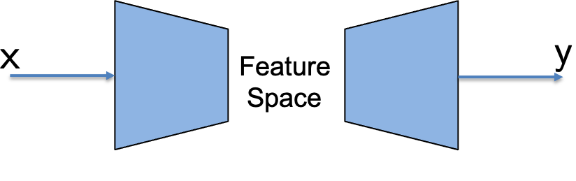 | 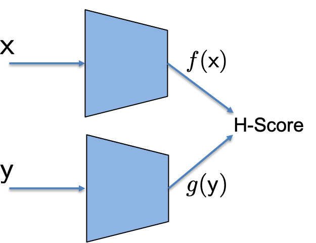 |
|---|---|
| Conventional Neural Network | H-Score Network |
\(\blacktriangle\) Demo 1: H-score Network
Here is a colab demo of how to implement an H-score network to learn the first mode, where the learned features are compared with theoretical results.
H-score Network, Conventional Neural Network, and SVD
At this point, we have made connections between three different problems:
- the modal decomposition problem, which is equivalent as a SVD of the \(\mathrm{PMI}\) function,
- the conventional neural networks, especially when we use the cross entropy loss) to train a classifier,
- the H-score network.
With the local approximation, all three problems have the same or equivalent objective function. The SVD requires ordered orthonormal features, and the other two do not. In exchange, both neural-network-based options are more suitable for working with data than directly with the probability model.
Compared with the normal neural networks, the H-score network method has a number of conceptual and practical advantages, which we will discuss now.
Feature Space Operations
Conceptually, the H-score network is a more appealing setup as it turns the objective of the system from learning a probability model to learning feature functions. For a specific inference task, we sometimes do not have a clear way to choose the metric to measure the quality of the decisions. There are many options for the loss metric to choose from, such as the cross entropy loss and the MSE loss with various regulators. When training a neural network, we are using task-specific metrics to encourage the chosen features to carry the “right” information.
In contrast, the H-score directly measures the quality of the information carried by the features. This helps to separate the learning of information features and how to use these features, or the information they carry, to make decisions.
One of the benefits of this separation is that the feature functions can be reused for other purposes. An immediate example is that after learning the \(\underline{f}^\ast, \underline{g}^*\) above, we can assemble these features in both
\[\begin{align*} {P}_{\mathsf{y|x}} \approx P_{\mathsf{y}} \cdot \left(1 + \underline{f}^\ast \otimes \underline{g}^\ast\right) \qquad \mbox{ and } \qquad P_{\mathsf{x|y}} \approx P_{\mathsf{x}} \cdot \left(1 + \underline{f}^\ast \otimes \underline{g}^\ast\right) \end{align*}\]as estimators in both directions.
It is worth mentioning that this shift from solving specific inference tasks to learning informative features is a widely accepted view in the literature under the names of “semantic information” or “representation learning,” etc.
Weak Dependence and Large Alphabets
Another reason for the importance of the above separation is that in some applications, the reconstruction quality is not a meaningful metric and thus cannot be used to encourage the learning of informative features.
A rather common situation is when the alphabet \(\mathcal{X}, \mathcal{Y}\) are both quite large, yet the dependence between \(\mathsf{x}\) and \(\mathsf{y}\) is rather weak. Put this in an example, consider two episodes of the “Star Wars” movies: the common theme between the two movies is obvious, but it would be pointless if we want to reconstruct one entire movie from the other one. Thus, it would be difficult if we use one movie as the input \(\mathsf{x}\) of a neural network and try to predict the other movie as the output \(\mathsf{y}\). On the other hand, training an H-score network to find correlated features of the two movies can find meaningful results.
We use the following experiment to demonstrate this point. Of course, we do not work with movies, but only synthetic time-sequences for the experiments.
\(\blacktriangle\) Demo 2: H-score for Sequential Data
Here is a colab demo to demonstrate how we apply H-score network to learn the dependence structure among high-dimensional data. Again, we generate the dataset from given probability laws to help us analyze the trained results and compare them with theoretical optimal values. However, unlike previous demos where \(\sf x\) and \(\sf y\) are categorical, here \(\sf x\) and \(\sf y\) are both sequences, and the cardinalities \(\vert\mathcal{X}\vert\), \(\vert\mathcal{Y}\vert\) are way larger than the sample size.
Flexible Control of Feature Functions
The most significant advantage of the H-score network is it allows flexible control of the learning of feature functions. We will use a few posts to discuss various ways of taking this advantage to solve more involved learning problems. At a glance, the obvious reason for this flexibility is that the feature functions are separated into individual modules in H-sore networks. This makes it easy to change individual feature functions according to the specific situation. In extreme cases, we might know one of the feature functions from domain knowledge and thus do not have to learn that function. It turns out that this flexibility opens up an entire line of work on feature space operations. Since the feature functions are the new information carriers, these operations will become the new “atomic operations” used in a wide range of problems.
Going Forward
H-score networks are our first step in processing based on modal decomposition. It offers some moderate benefits and convenience in the standard bi-variate “data-label” problems. To us, it is more of a conceptual step, where our focus of designing neural networks is no longer to predict the labels but rather shifted to designing the feature functions since our loss metric is now about the feature functions. In a way, this is better aligned with our goals since these features are indeed the carriers of our knowledge, and we would often need to store, exchange, and even use these features for multiple purposes in the more complex multi-variate problems.
In our next step, we will develop one more tool to directly process the feature functions, which is, in a sense, to make projections in the functional space using neural networks. This will be a useful addition to our toolbox before we start to address multi-variate learning problems.
This post is based on the joint work with Dr. Xiagxiang Xu.
Enjoy Reading This Article?
Here are some more articles you might like to read next: