The Nested H-Score Network
The Key Points
In our previous posts, we started to develop a geometric view of the feature extraction problem. We started with the geometry of functional spaces by defining inner products and distances and then relating the task of finding information-carrying features to finding approximations of functions in this space. Based on this approach, we proposed the use of the H-Score networks as one method to learn informative feature functions from data using neural networks. In this post, we describe a new architecture, the nested H-Score network, which is used to make projections in the functional space with neural networks. Projections are perhaps the most fundamental geometric operations, which are now made possible and efficient through the training of neural networks. We will show some examples of how to use this method to regulate the feature functions, incorporate external knowledge, and prioritize or separate information sources, which are the critical steps toward multi-variate and distributed learning problems.
 |
| H-Score Network |
Previously
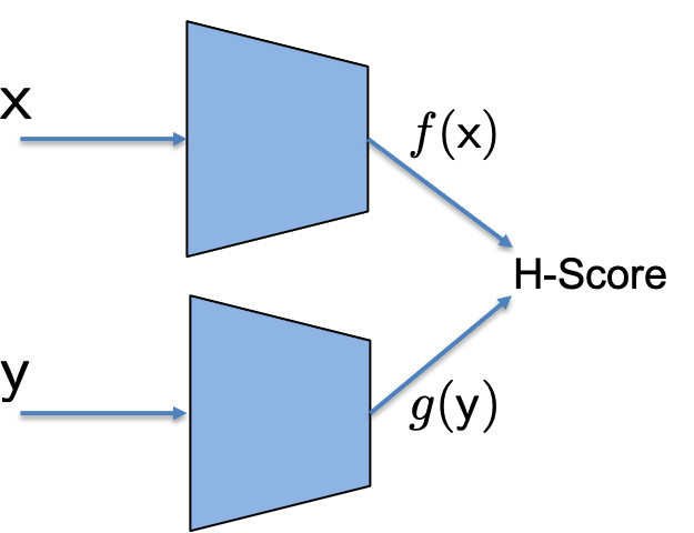
In this page, we defined H-Score network as shown in the figure, where the two sub-networks are used to generate features of \(\mathsf x\) and \(\mathsf y\): \(\underline{f} \in \mathcal {F_X}^k, \underline{g}\in \mathcal {F_Y}^k\). The two features are used together to evaluate a metric, the H-score,
\[\mathscr{H}(\underline{f}, \underline{g}) =\mathrm{trace} (\mathrm{cov} (\underline{f}, \underline{g})) - \frac{1}{2} \mathrm{trace}(\mathbb E[\underline{f} \cdot \underline{f}^T] \cdot \mathbb E[\underline{g} \cdot \underline{g}^T])\]where the covariance and the expectation are evaluated by the empirical averages over the batch of samples. We use back-propagation to train the two networks to find
\[\underline{f}^\ast, \underline{g}^\ast = \arg\max_{\underline{f}, \underline{g}} \; \mathscr{H}(\underline{f}, \underline{g}).\]The resulting optimal choice \(\underline{f}^\ast, \underline{g}^\ast\) is promised to be a good set of feature functions. They are the solutions of the approximated and unconstrained versions of the modal decomposition problem, which has a connection to a number of theoretical problems, and, in a short sentence, picks “informative” features.
The H-Score network is different from the modal decomposition problem in the following ways:
- Approximation:
- Neural networks can have limited expressive power and imperfect convergence;
- The use of finite sample batches introduces randomness in the empirical averages and generalization error;
- We use a local approximation when formulating the modal decomposition. For the rest of this page, we will take the local approximation for granted. For example, we will not distinguish between the function \(\mathrm{PMI}_{\mathsf {xy}} = \log \frac{P_{\mathsf {xy}}}{P_\mathsf x\cdot P_\mathsf y} \; \in \; \mathcal {F_{X\times Y}}\) and its approximation \(\widetilde{\mathrm{PMI}}_{\mathsf {xy}} = \frac{P_{\mathsf {xy}} - P_{\mathsf x}\cdot P_{\mathsf y}}{P_\mathsf x\cdot P_{\mathsf y}} \; \in \; \mathcal {F_{X\times Y}}\). $$
- Constraints: in the formulation of modal decomposition, we restricted the feature functions to satisfy a set of constraints that the features are all normalized, orthogonal to each other, and that they are organized in descending order in correlation coefficients. A detailed discussion can be found here.
The goal of this post is to develop a new architecture to put these missing constraints back in the learning process. By doing that, we also introduce a systematic way to inject controls into the learning with H-score networks.
Nested H-Score Network
We start by consider the following problem to extract a single mode from a given model \(P_{\mathsf {xy}}\), but with a simple constraint: for a given function \(\bar{f}: \mathcal X \to \mathbb R\), we would like to find a mode, i.e. a pair of features \(f(\cdot), g(\cdot)\), to be the optimal rank-$1$ approximation as before, but under the constraint that \(f \perp \bar{f}\), i.e. \(\mathbb E_{\mathsf x \sim P_\mathsf x}[f(\mathsf x) \cdot \bar{f}(\mathsf x)] = 0\):
\[(f^\ast, g^\ast) = \arg\min_{\small{\begin{array}{l}(f, g): f\in \mathcal {F_X}, g \in \mathcal {F_Y}, \\ \quad \mathbb E[f(\mathsf x)\cdot \bar{f}(\mathsf x)]=0\end{array}}} \; \left\Vert \mathrm{PMI} - f \otimes g \right\Vert^2\]where \(\mathrm{PMI}\) is the point-wise mutual information function with \(\mathrm{PMI} (x,y) = \log \frac{P_{\mathsf {xy}}(x,y)}{ P_\mathsf x(x)P_\mathsf y(y)}\), for \(x\in \mathcal X, y \in \mathcal Y\).
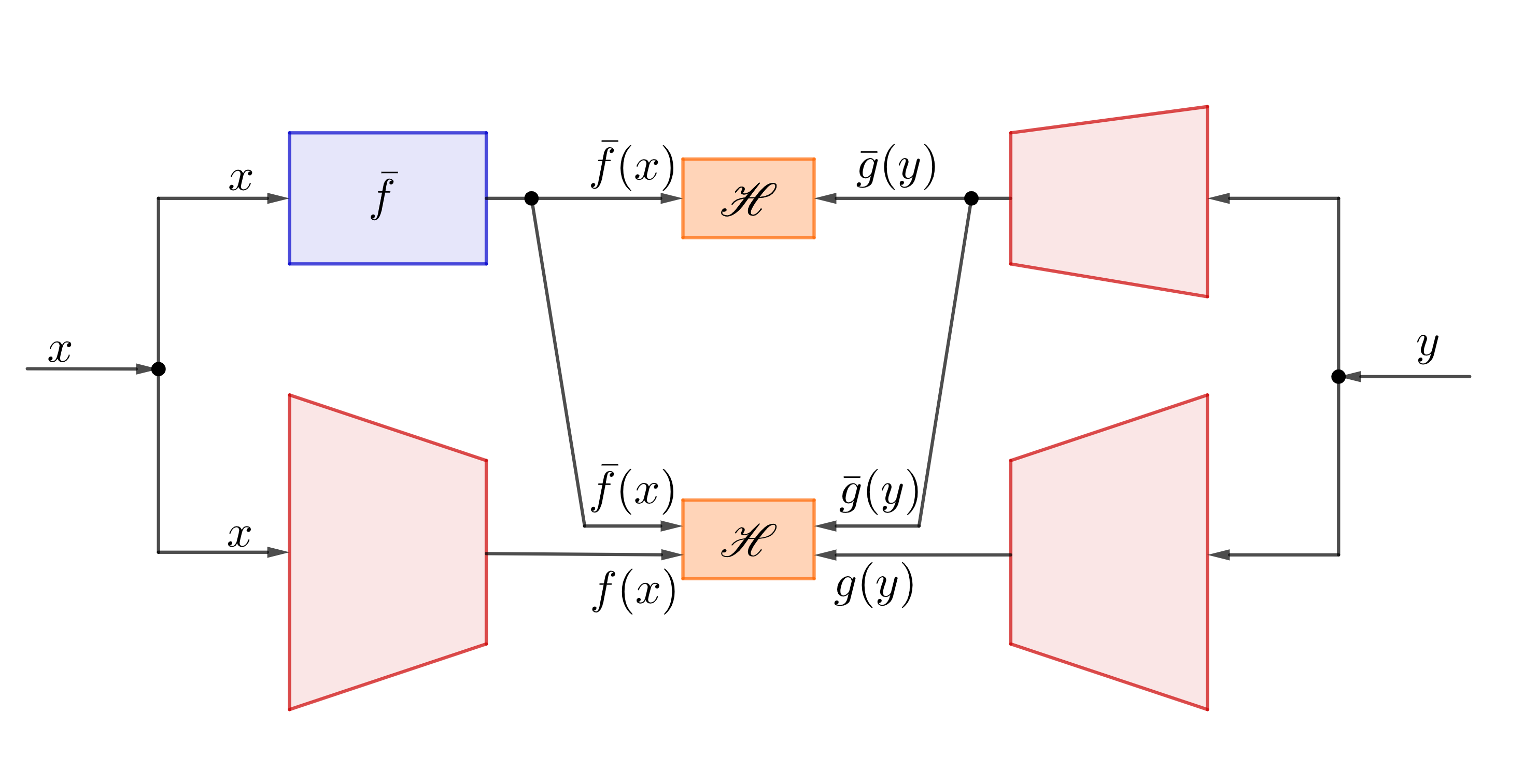 |
| Nested H-Score Network to find features orthogonal to a given $\bar{f}$ |
While there are many different ways to solve optimization problems with constraints, the figure shows the nested H-Score network we use, which is based on simultaneously training a few connected neural networks.
In the figure, the blue box \(\bar{f}\) is the given function that the chosen feature function needs to be orthogonal to. The three red sub-networks are used to generate \(1\)-dimensional feature functions \(\bar{g}, f\) and \(g\). (As we will see soon, that \(f\) and \(g\) can, in fact, be higher dimensional, hence drawn slightly bigger in the figure.)
With a batch of samples \((x_i, y_i), i=1, \ldots, n\), the network is trained with the following procedure.
Training for Nested H-Score Networks
- Each sample pair \((x_i, y_i)\) is used to compute \(\bar{f}(x_i)\), and forward pass through the neural networks to evaluate \(f(x_i), \bar{g}(y_i), g(y_i)\);
- The output \(\bar{f}(\mathsf x_i), \bar{g}(\mathsf y_i), i=1, \ldots, n\) are used together to evaluate the H-score for \(1\)-D feature pairs shown on the top box; the two pairs of features \([\bar{f}, f]\) and \([\bar{g}, g]\) are used to evaluate a 2-D H-score in the lower box. In both cases, the expectations are replaced by the empirical means over the batch;
- The gradients to maximize the sum of the two H-scores are back-propagated through the networks to update weights. Because of the separation of the neural network modules, the sum of the gradients from the two H-scores is used to train \(\bar{g}\); only the gradients from the bottom H-score are used to train \(f\) and \(g\) networks.
- Iterate the above procedure until convergence.
To see how this achieves the goal, it might be easier to look at a slightly different way to train the network, namely the sequential training. Here, we first only use the top H-Score to train the feature function \(\bar{g}\). From the definition of the H-Score, we know this finds \(\bar{g}^\ast\) by solving the following optimization.
\[\begin{align} \bar{g}^\ast = \arg \min_{\bar{g}} \; \left\Vert\mathrm{PMI} - \bar{f} \otimes \bar{g}\right\Vert^2 \end{align}\]After that, we freeze \(\bar{g}^\ast\), and use the bottom H-Score to train both \(f\) and \(g\). With this choice of \(\bar{g}^\ast\), we have that the minimum error, \(\mathrm{PMI} - \bar{f} \otimes \bar{g}^\ast\) must be orthogonal to \(\bar{f}\) in the sense that for every \(y\), \(\mathrm{PMI}(\cdot, y)\) as a function over \(\mathcal X\) is orthogonal to \(\bar{f}\), since otherwise the L2 error can be further reduced. The maximization of the bottom H-Score is now the following optimization problem:
\[\begin{align} (f^\ast, g^\ast) = \arg\min_{f, g} \; \left\Vert \mathrm{PMI} - (\bar{f}\otimes \bar{g}^\ast + f\otimes g) \right\Vert^2 \end{align}\]This can be read as the rank-\(1\) approximation to \((\mathrm{PMI}- \bar{f}\otimes \bar{g}^\ast)\), which is orthogonal to \(\bar{f}\). So the resulting optimal choice of \(f^\ast\) must also be orthogonal to \(\bar{f}\) as we hoped.
A few remarks are in order now.
-
One should check that at this point if we freeze the choice \(f^\ast, g^\ast\) and allow \(\bar{g}\) to update, \(\bar{g}^\ast\) defined in (1) actually maximizes both H-Scores. Thus if we turn the sequential training into iteratively optimized \(\bar{g}\) and \(f, g\), we get the same results.
-
In practice, we would not wait for the convergence of one step before starting the next, and thus the proposed training procedure is what we call simultaneous training, where all neural networks are updated simultaneously. It can be shown that in this setup, the results are the same as those from the sequential training. However, in our later examples of using the nested H-Score architectures, often with subtle variations, we need to discuss in each case whether this still holds.
-
There are, of course, other ways to make sure the learned feature function is orthogonal to the given \(\bar{f}\). For example, one could directly project the learned feature function against \(\bar{f}\). Here, the projection operation is separated from the training of the neural network, raising the issue that the objective function used in training may not be perfectly aligned with that in the space after the projection. In nested H-Score networks, the orthogonality constraint is naturally included in the training of the neural networks. There is also some additional flexibility with this design. For example, in several follow-up cases using nested H-Score, we would learn \(\bar{f}\) from data at the same time.
Example: Ordered Modal Decomposition
We now go back to the problem that motivated this study: we would like to use the nested H-Score network to solve the modal decomposition problem. That is, we want to find \(k\) feature pairs that not only form a good low-rank approximation to the model but hope the extracted feature functions to be orthonormal and the modes to be in descending order of strengths.
We would like to emphasize the importance of this step: we are deviating from the standard operation of neural networks, which generate feature functions that are in the form of an arbitrary linear combination of the standard orthonormal and ordered modes. This is one key reason that the learning results of neural networks have little hope of allowing any interpretation. Sorting out the features in a standard form is an important starting point if we want to control, measure, and reuse the learned features.
As we will use the nested structure repeatedly, to avoid having too many lines in our figures, we will adopt a new concatenation symbol, “\(\,+\hspace{-.7em}+\,\)”, where simply takes all the inputs to form a vector output. In some drawings, such an operation to merge data is simply denoted by a dot in the graph, but here, we use a special symbol to emphasize the change of dimensionality. For example, the concatenation operation in the nest H-Score network is replaced with a new figure as follows.
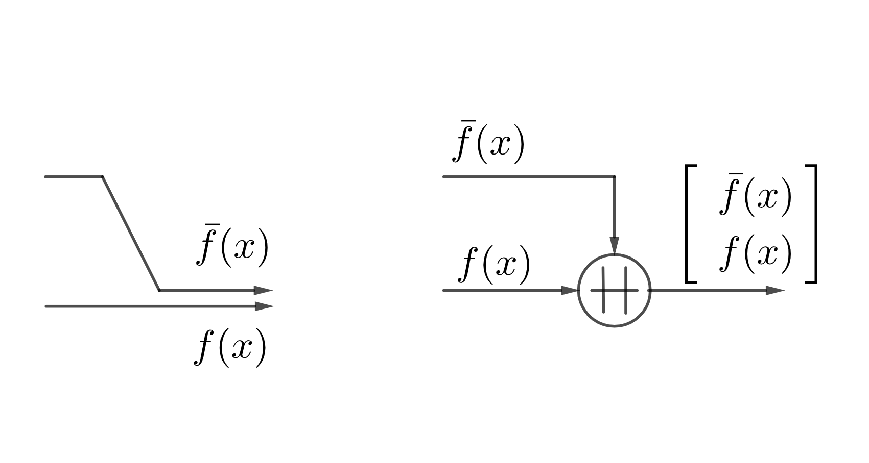 |
| The Concatenation Symbol |
Now the nested H-Score network that would generate orthogonal modes in descending order is as follows.
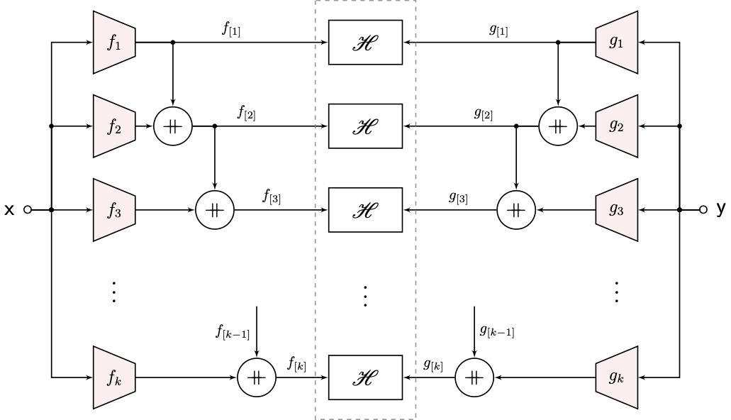 |
| Nested H-Score Network for Ordered Modal Decomposition |
In the figure, we used the notation \(f_{[k]} = [f_1, \ldots, f_k]\). Again, it is easier to understand the operation from sequential training. We can first train the \(f_1, g_1\) block with the top H-Score box, and this finds the first mode \(f^\ast_1, g^\ast_1 = \zeta_1(P_{\mathsf {xy}})\). After that, we train \(f_2, g_2\) with the first mode frozen. The nested network ensures that the resulting mode is orthogonal to the first mode, which by definition is the second mode \(\zeta_2(P_{\mathsf {xy}})\). Following this sequence, we can get the \(k^{th}\) mode that is orthogonal to all the previous \(k-1\) ones. It takes proof to state that we can indeed simultaneously train all sub-networks, which we omit from this page.
\(\blacktriangle\) Pytorch Implementations
The first Colab demo illustrates how to implement a nested H-score network in PytTorch, where we compare the extracted modes with the theoretical results.
As in the previous post, we can also apply the nested H-score on sequential data. In the second demo, we compare the nested H-score with the vanilla H-score, which also demonstrates the impact of feature dimension.
Going Forward
Nested H-Score Networks are our way to make projections in the space of feature functions using interconnected neural networks. This is a fundamental operation in the functional space. In fact, in many learning problems, especially when the problem is more complex, such as with multi-modal data, multiple tasks, distributed learning constraints, time-varying models, privacy/security/fairness requirements, or when there is external knowledge that needs to be incorporated in the learning, such projection operations become critical. In our next post, we will give one such example with a multi-terminal learning problem.
This post is based on the joint work with Dr. Xiagxiang Xu.
Enjoy Reading This Article?
Here are some more articles you might like to read next: