Symbol Detection in Wireless Communication
The Key Points
In our previous developments, we introduced the H-score network, which is a way to learn informative features from datasets, similar to a normal neural network but was claimed to be more flexible. In this post, we use a concrete example of wireless communications to demonstrate this flexibility. In a nutshell, the advantage of our solution comes from changing the objective from learning to solve a specific inference task to learning feature functions that carry information that can be reused and combined with other sources of information. We demonstrate that this approach can help us to design neural-network-based solutions not to a single case but a parameterized set of cases, as required by this specific engineering problem. We use this example to discuss the general methodology of integrating learning modules into engineering solutions.
Previously
This post is based on a sequence of previous posts. We briefly summarize the main points that we will be using here.
In Modal Decomposition, we stated that the dependence between two random variables, \(\mathsf{x, y}\) can be decomposed into a sequence of correlation between feature pairs \(f_i(\mathsf{x}), g_i(\mathsf{y}), i=1, 2, \ldots\). These feature functions are defined using the following optimization:
\[\underline{f}^\ast, \underline{g}^\ast = \arg\min_{\substack{\underline{f} \in \mathcal {F_X}^k \\ \underline{g} \in \mathcal {F_Y}^k}} \; \Vert \mathrm{PMI}_{\mathsf{x,y}} -\underline{f} \otimes \underline{y}\Vert^2\]where \(\mathrm{PMI}_{\mathsf{x,y}} = \log \frac{P_{\mathsf{xy}}}{P_{\mathsf{x}} P_{\mathsf{y}}}\) is the point-wise mutual information function; \(\underline{f} = [f_1, \ldots, f_k], \underline{g} = [g_1, \ldots, g_k]\) are two collections of orthonormal feature functions with correlation \(\sigma_i = \rho (f_i(\mathsf{x}), g_i(\mathsf{y}))\) in a descending order.
 |  |
| H-Score Network | Nested H-Score Network to find features orthogonal to a given \(\bar{f}\) |
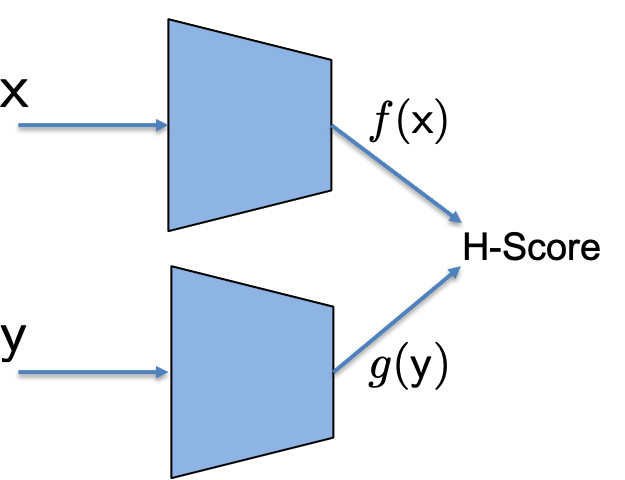
In H-score, we defined a new metric called the H-score:
\[\mathscr{H}(\underline{f}, \underline{g}) =\mathrm{trace} (\mathrm{cov} (\underline{f}, \underline{g})) - \frac{1}{2} \mathrm{trace}(\mathbb E[\underline{f} \cdot \underline{f}^T] \cdot \mathbb E[\underline{g} \cdot \underline{g}^T])\]and a network architecture called the H-score network, as shown in the figure, where we can learn the informative features defined in the modal decomposition by maximizing the H-score with a given dataset.
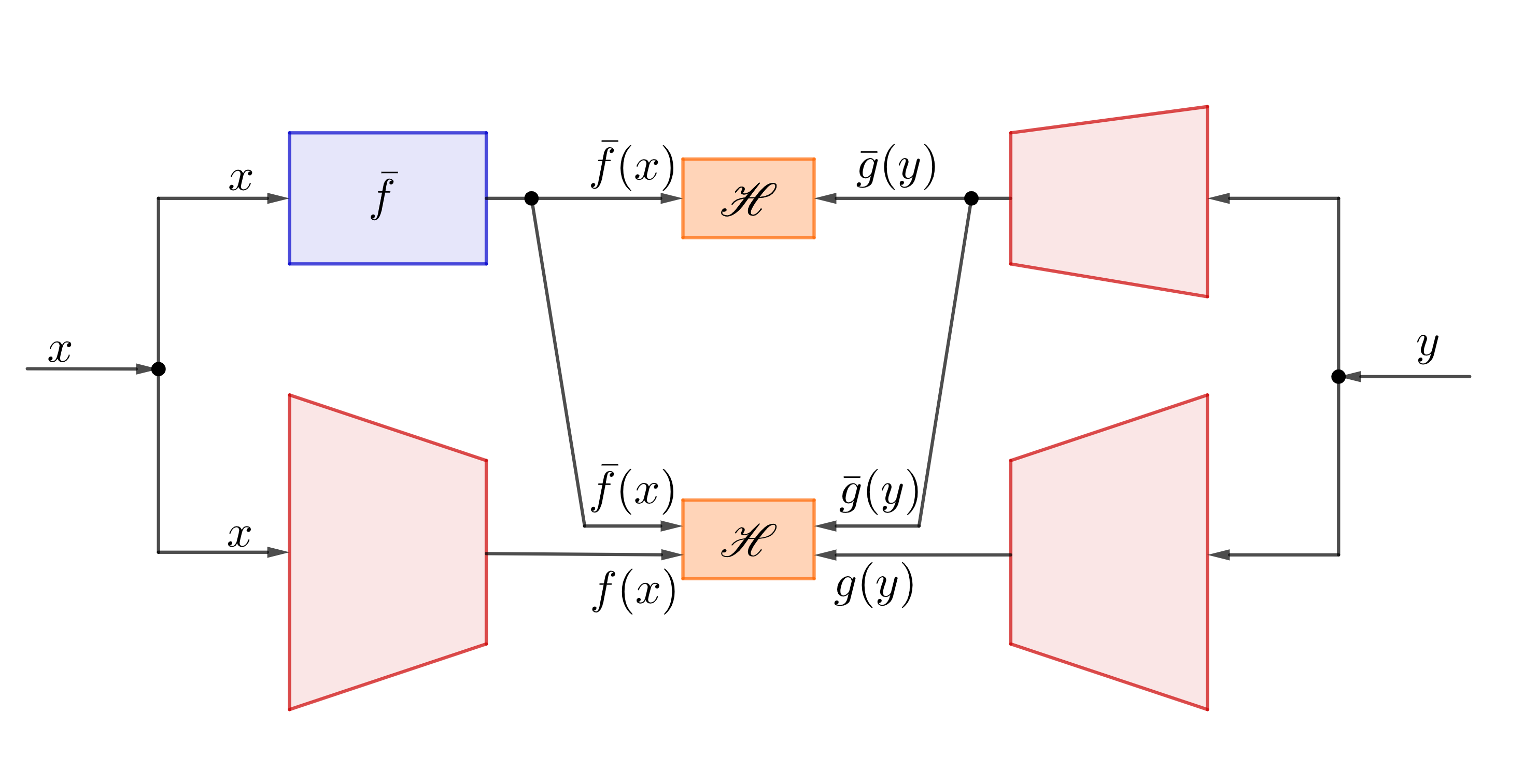
In nested H-score network, we introduced a nested architecture, see figure, to enforce orthogonality constraints in the learning process.
The main point of this sequence of works is to introduce the key concepts and building blocks of feature-centric learning, where we view feature functions as the basic carrier of information and turn the learning objective from making a certain decision to finding feature functions that carry specific information. This general method makes the learning procedure more controllable and the learning results reusable. The H-score can be viewed as a quality metric for features. The nested H-score network can be viewed as a numerical method for the basic projection operation of features. Both are needed for further development.
A Wireless Communication Problem
 |
| A Wireless Fading Interference Channel |
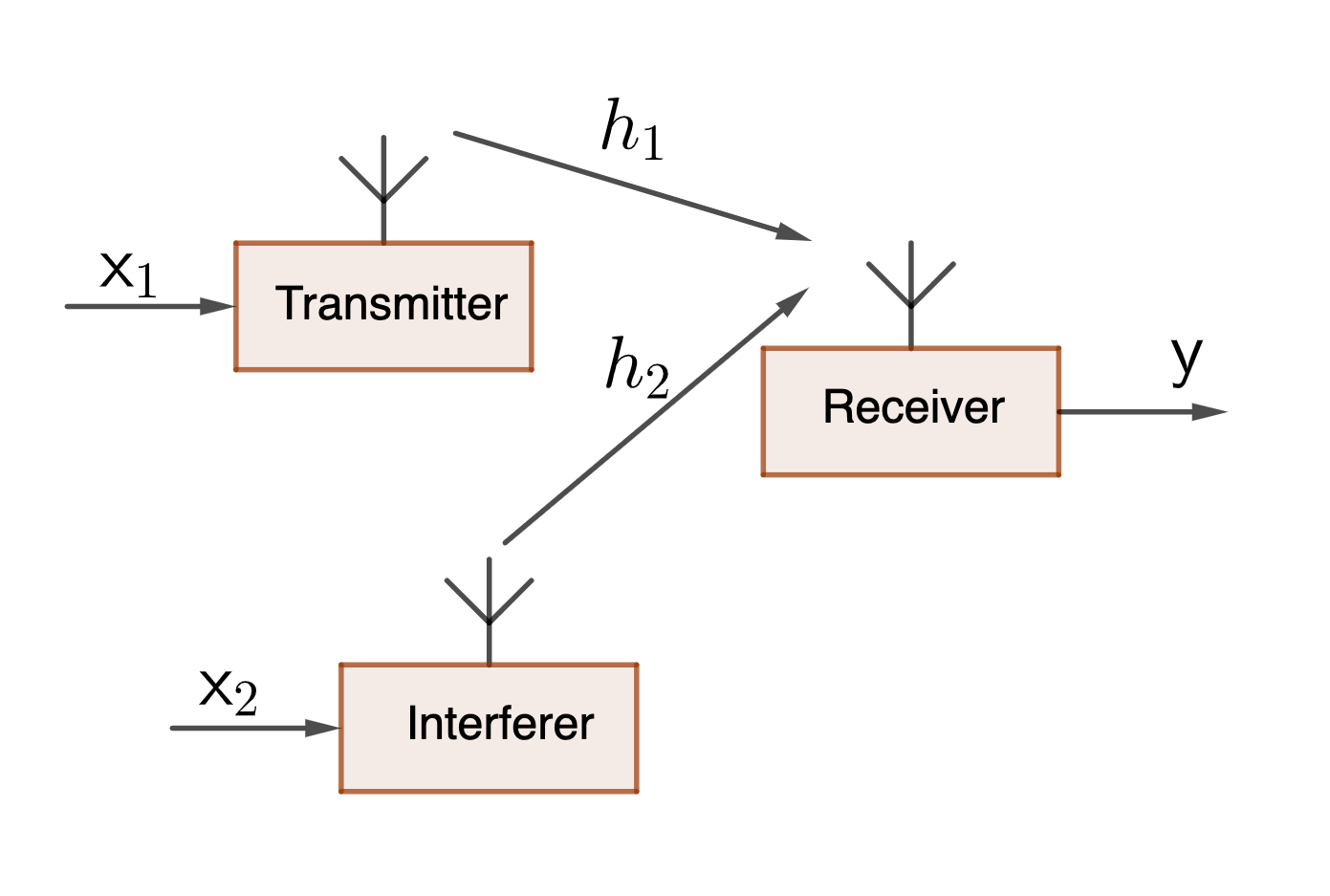
The problem we are working on is called “symbol detection in fading interference channel,” which is a classic problem in wireless communications. For a more complete reference, here is a wonderful textbook. Roughly the idea is depicted in the figure: a transmitter tries to send a symbol \(\mathsf {x}_1\) to the receiver, but there is another transmitter, the interferer, which is transmitting his signal at the same time. Thus, the receiver receives a signal \(\mathsf y\) which is a mixture of both the desired signal \(\mathsf {x}_1\) and the interfering signal \(\mathsf {x}_2\), with some additive noise introduced by the receiver circuits. The goal is to design a receiver processing that can figure out the value of the desired signal \(\mathsf {x}_1\).
Mathematically, the received signal can be written as
\[\mathsf{y} = h_1 \cdot \mathsf{x}_1 + h_2 \cdot \mathsf{x}_2 + \mathsf {w}\]where
- Because all the symbols are transmitted at a carrier frequency, it is conventional to think of all the variables as complex-valued. Here, we have assumed the standard approach to isolate a single group of transmitted and received symbols. Thus, all the variables are complex scalars in \(\mathcal C\).
- \(h_1, h_2\) are called the fading coefficients for the two corresponding channels. These are usually random, depending on the position of the transmitter and the receiver, and the environment around them. If the transmitter moves, these fading coefficients can change over time, too. However, a wireless system usually has a separate procedure to estimate these coefficients. So, these coefficients are considered as known side information at the receiver, called the channel state information (CSI).
- \(\mathsf w\) is complex Gaussian distributed, independent of all the other variables. This is usually referred to as the “additive Gaussian noise”. If there is no interference, the received signal can be described with a conditional distribution of \(\mathsf y\) given \(\mathsf {x}_1\), which is Gaussian distributed with a mean of \(h_1 x_1\). The decision of what symbol \(\mathsf{x}_1\) is transmitted is now a standard hypothesis testing problem, with Gaussian noise, for which the MAP decision is simple and the optimal solution.
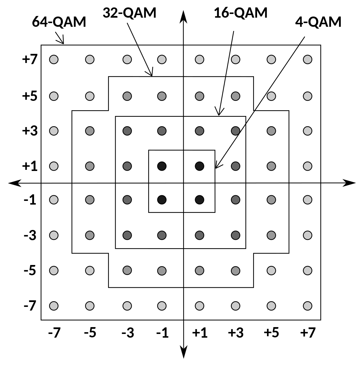
- What makes these problems interesting is that the transmitted signals \(\mathsf{x}_1\) and the signal transmitted by the interferer \(\mathsf{x}_2\) are both digital signals, in the sense that they are chosen from a discrete set of possible values on the complex plane, which is called a constellation. The most commonly used one is called the QAM.
 |
| Michel Bakni, CC BY-SA 4.0 https://creativecommons.org/licenses/by-sa/4.0, via Wikimedia Commons |
In this post, we will assume that \(\mathsf{x}_1\) is equally likely chosen from a binary alphabet \(\mathsf{x}_1 \in \{+1, -1\}\); and the interference symbol \(\mathsf{x}_2\) is chosen uniformly from a 16-QAM constellation, which, as shown in the figure, are the 16-point regular grid around the origin.
This is obviously a special and simple case, but it is sufficient to make our points. We are interested only in detecting the value of \(\mathsf{x}_1\), which is a binary decision. However, because of the interference signal, our received signal \(\mathsf {y}\) is corrupted with non-Gaussian noise.
To see how this works, consider an example shown in the following figure:
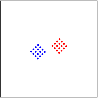 |
| A “good” case of interference |
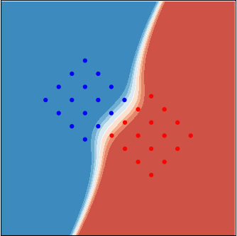
Here, we use the color “red” for \(\mathsf{x}_1 = +1\), and “blue” for \(\mathsf{x}_1=-1\). When we transmit \(\mathsf{x}_1= +1\), the interferer transmits a randomly independently chosen point in his 16-QAM constellation. This causes the noiseless signal \(h_1 \mathsf{x}_1 + h_2 \mathsf{x}_2\) to be one of the \(16\) red dots in the figure. If we transmit \(\mathsf{x}_1 = -1\), this signal before adding noise is one of the \(16\) blue dots. The additive noise \(\mathsf {w}\) is then added to the chosen dot, which makes the received symbol \(\mathsf{y}\) to be somewhere around.
Our goal is to observe the received symbol \(\mathsf{y}\) and decide whether it was a red or a blue dot transmitted. Mathematically, the decision is between two mixed Gaussian distributions. The case shown above is considered a “good” case with weak interference. That is, even with the interference, the red and the blue cases are rather separable. As long as the additive noise \(\mathsf {w}\) is not too large, one can simply draw a line to separate the red and the blue cases rather well. In fact, most of the current commercial wireless communication systems use linear decision functions. That is, a straight line is drawn in this figure to separate the red and the blue.
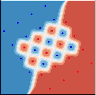
Unfortunately, the configuration of these “dots” is determined by the fading coefficients \(h_1, h_2\), which we can observe but cannot control. There is a small probability that the fading can take values that cause an “undesirable” situation. A few such cases are shown below. If the interference is strong, the two groups of dots can be “interleaved,” making it rather difficult to separate them. Furthermore, depending on the value of the fading coefficients, these cases with strong interference can be rather different, as shown in the figure. That is, we cannot design a decision-maker for one case and use it for another case.
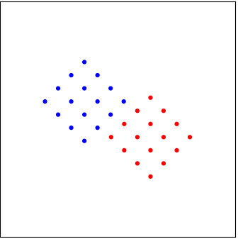 | 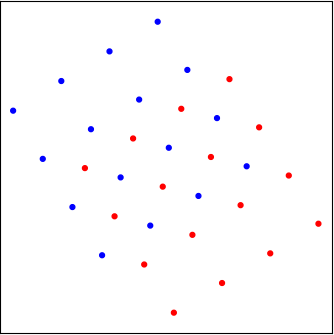 | 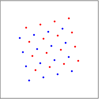 |
| A “marginal” case of interference | A case with strong interference | A different case with strong interference |
Why is this difficult?
Analytically, the optimal decision using the likelihood ratio test (LRT) is not difficult to find. The likelihood function of both the red and the blue cases are simply mixture-Gaussian densities: the average of \(16\) equally weighted Gaussian densities. The log-likelihood ratio function can be rather non-linear. Examples are shown in the figure, respectively, corresponding to the \(3\) cases above. The color code represents the scalar value of this function: red for positive values, which means \(\mathsf{x}_1=+1\) is more likely, and blue for \(\mathsf{x}_1=-1\). A simple threshold test can cut out the decision regions.
 |  | 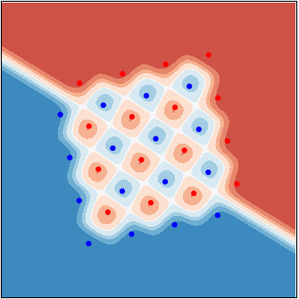 |
| Case 1 | Case 2 | Case 3 |
In practice, however, this analytically optimal decision is rarely implemented for some practical reasons. One of them is the lack of non-linear processing circuits in conventional wireless communication devices. Neural networks, as a general-purpose non-linear processor, are now widely used in handheld wireless devices. This makes neural-network-based solutions to this problem an attractive possibility.
The immediate difficulty in building a decision-maker with a neural network is the lack of training samples. In this application, we can have both off-line training and on-line training. Offline training samples can be simulated in the wireless environment based on the industry’s extensive channel measurement results. The problem is that there are infinitely many possible situations, as the fading coefficients \(h_1, h_2\) in our example, are continuous-valued. Thus, whichever specific environment or collection of environments we simulate, the online situation is inevitably different. Online training, on the other hand, is more targeted to the case of interest but is much more expensive. Every symbol we use for training is a symbol we cannot use to carry the communication payload. The wireless channel also changes quite fast over time as mobile users move, making online training results expire.
Another difficulty in this problem is the high accuracy requirement. Symbol detections in wireless communication systems require the error rate to be around \(10^{-3}\). Situations like cases 2 and case 3 in both figures are said to have strong interference, which occurs with a probability of the order of \(10^{-2}\). This means a good receiver needs to do well in all the nice cases like case 1, but what really defines a good receiver is how it handles the strong interference cases. As a result, using the average performance as the objective to train the neural network is not a good idea: how a receiver acts in difficult cases may not count much in the average performance and do not have enough samples in a reasonable-sized training set.
Why is this a common problem?
The reason that we like this symbol detection problem is because it is a very typical case for using neural networks in engineering problems. There is clearly a potential for remarkable performance gain, which can come from
- The use of neural networks in the place of specialized non-linear circuits;
- The training that allows the system to adapt to specific environments.
The difficulties are also clear:
- the situations where we want to use the neural networks are almost always different from those we have in the training set;
- what we hope to get from the neural networks is not just the optimal solution in one specific case but a collection of optimal solutions controlled by parameters (in this example, the channel coefficients.)
- we also have knowledge of specific structures of the data (for example, the repetitive patterns in the above plots,) which we hope to “tell” the neural network so it does not require more samples to learn this known fact.
At a higher level, the issue is that neural networks are often operated as black boxes. In engineering problems, there is often the need to inject external domain knowledge into the neural networks in order to control the learning procedure, impose restrictions on learning results, reuse learning results as the environment changes, and reduce the overall learning costs.
The goal of this page is to develop a generic solution to this family of problems. Since the goal is to reach into the internal operations of neural networks, the H-score networks, which are based on the concept of decomposition of probability models, is a useful tool.
A solution using nested H-score networks
We write the channel state information as one random variable \(\mathsf{s} = [h_1, h_2]^T\). We write the target random variable, i.e., the one we would like to make a decision on, as \(\mathsf {x} = \mathsf {x}_1 \in \{0, 1\}\). We write the observed variable as \(\mathsf{y}\), and include the randomness from the interfering signal \(\mathsf{x}_2\) in the conditional distribution \(P_{\mathsf{y\vert x, s}}\). With these notations, the probability law that is relevant to this problem is the 3-way dependence of \(\mathsf{x, y, s}\).
In the literature of wireless communications, a standard way to work with such a multi-variate dependence is by using the chain rule.
\[I(\mathsf{y; (x, s)}) = I(\mathsf{y;s} ) + I(\mathsf{y;x|s}),\]The quantity of interest is \(I(\mathsf{y;x\vert s})\), which is maximized by choosing the optimal distribution of \(\mathsf{x}\) and a corresponding coding scheme. The resulting maximum of this conditional mutual information is called the coherent capacity of the channel.
The point is we would like to separate the contribution of \(\mathsf{x}\) and that of \(\mathsf{s}\) in the three-way dependence. This is a problem we have just studied in the previous post. The key is to use a nested H-score network, as shown below, to make this separation computationally.
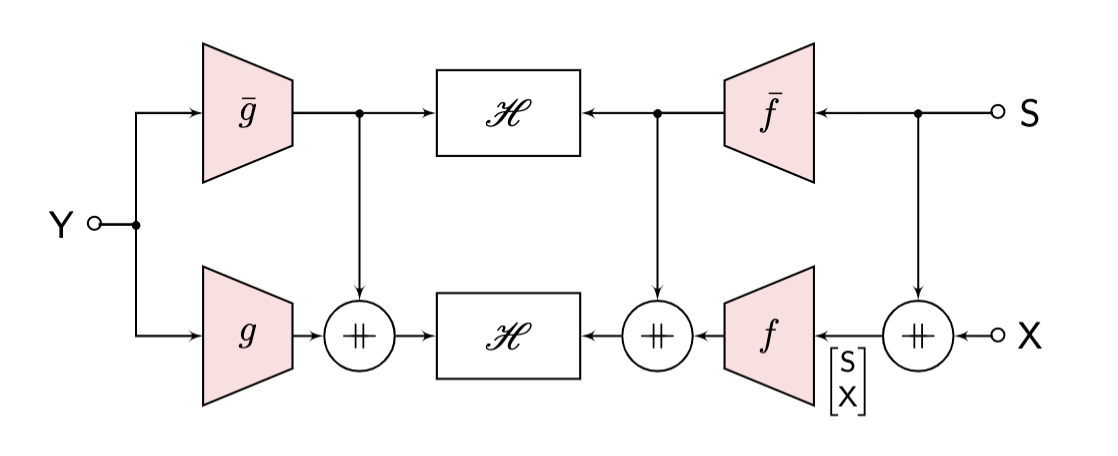 |
| Nested H-Score Network for Learning with Side Information |
The assembling step
Different from the common procedure of training a neural network and use it in the same place, here, we need an extra assembling step to connect the trained feature function modules into the desired decision maker.
After training the nested H-score network above, we have four modules \(f, g, \overline{f}, \overline{g}\), with the following meanings
\[\begin{align*} P_{\mathsf{y,s}} &\approx P_{\mathsf{y}} \cdot P_{\mathsf{s}} \cdot \left(1 + \overline{f} \otimes \overline{g}\right)\\ P_{\mathsf{y,s,x}} &\approx P_{\mathsf{y}} \cdot P_{\mathsf{s}} P_{\mathsf{x}} \cdot \left(1 + \overline{f} \otimes \overline{g} + f \otimes g\right) \end{align*}\]We need a simple step of using the Bayes rule to get an approximated version of
\[P_{\mathsf {x \vert s,y}} = \frac{P_{\mathsf{y,s,x}}}{P_{\mathsf{y,s}}}\]which can be used as the decision maker: use \(\mathsf{y}\) and \(\mathsf{s}\) as inputs, we can decide which value of \(\mathsf{x}\) is more likely.
We emphasize here that the extra assembling step is the direct consequence of training not to learn a specific decision-maker, but to learn the useful features. This allows the learned feature modules to be evaluated and reused in different problems. This procedure is a key step to move away from task-specific learning and toward learning reusable information contents. It is also a key step in breaking the blackbox of end-to-end training.
\(\blacktriangle\) Demo: Pytorch implementation
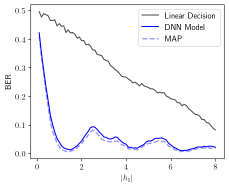
Here is a code for this experiment. The key performance result given in the following figure compares the current state-of-art decision after linear processing, the proposed solution based on the nested H-score network, and the theoretical optimal MAP decisions.
 |
| Performance Comparison between the Current and the Proposed Solutions |
We have two disclaimers:
- The training and the performance evaluation of this experiment both take some time. The training can be done offline, which is basically free for communication systems. The performance evaluation part is left in the experiment. Readers are recommended to select a subset to run.
- The above curve is plotted by fixing the strengths of the signal and the interference: \(\vert h_1\vert \in [0.0 .. 8.0], \vert h_2\vert =1\) at fixed values. This is not common for communication engineers. A more commonly used approach would choose signal strengths to be random, following certain distribution e.g. Rayleigh Fading, and make the plot with average interference strength. This plot is also included in our code. We choose to this one as it reveals the non-linear nature of the problem and the fact that the proposed solution can follow the non-linear behavior of the theoretical optimal solution quite well.
The Lessons
We take a little time to reflect on the lessons we learned through this experiment.
Good engineering solutions
We are quite happy with the final result of this experiment. It shows that we can indeed use neural-network-based solutions in very mature engineering problems. The symbol detection problem is a well-understood and widely used problem in the industry, with well-defined performance measures and benchmarks. It is also known to require very precise processing and has a very limited online computation budget. The fact that our solution can outperform the existing solutions, which run on everybody’s cell phone, is quite impressive.
The especially remarkable part is that by using the nested H-score network, our solution is optimal not for a single scenario but a parameterized sequence of scenarios, with our choice of the parameters as the channel state information. Our solution also shifted the computation requirement: we used extensive offline training, allowing us to have zero online retraining or re-adaptation beyond simply setting the CSI parameter to indicate which scenario we are in. These are all desired/required by the target application.
The separation: feature learning and assembling
A key conceptual change we propose with this sequence of blogs and experiments is the shift from learning for a specific inference task to learning information-carrying feature functions. This concept is analogous to the separation of source and channel coding in information theory. We believe this is a critical step to make training large neural networks, which consume vast amounts of data and computation, contribute to learning reusable knowledge.
There are two key technical components in such a conceptual shift. First, we can no longer rely on task-specific performance metrics to train the neural networks. Instead, a metric directly evaluating the information contents, on its quality and relevance, is needed in the training process. The geometric concept and the H-score in our works are for this purpose. Second, after training, there needs to be a separate assembling stage, where feature functions from different sources are put together to form a decision-maker. We also see this process in this experiment.
Going Forward: What is a “White Box Solution” ?
There are many discussions about “applying AI to specific domains” or “verticals.” These are, of course, correct visions for the future development that we embrace. The question is, how do we do that? How do we turn a black box solution into a white box solution? What exactly is interpretable learning? Does it count if we just add some metrics, maybe an information-theoretic metric, as a regulator in the training? This sequence of blogs tries to answer these questions by examples.
First, conceptually, we believe that fundamentally new information metrics are needed. In these learning problems, information carriers are no longer bits, and the information carried by a feature function should not only be measured by “how much information there is” but also by “what the information is about?”. A vector description of the information is thus needed. This concept is a fundamental extension of the classical information theory. We show in this series that such a concept leads to the definition of the H-score and a collection of new operations.
Second, at an operational level, we should expect concrete operations when we open a black box. We summarize them into the following three capabilities, which we call the “SET” capabilities.
-
Separable: When we train a neural network for a complex task, we should be able to extract its answer to a simple sub-task and know which part of the network is responsible for that answer. For example, if we can recognize a person from an image, we should know his/her gender or hair color; if we train a neural network to detect symbols from the received signal, then somewhere in the neural network, we must have an estimate of the channel state.
-
Exchangeable: We should be able to replace the answer of a large neural network to an element question with a different answer and still run the rest of the system, as a way to control the behavior of the overall system. We have seen such experiments as changing the gender of the object in an image. Our experiment changing the channel state information as a parameter is another example.
-
Transferrable: Here, we do not mean to train a large network with one dataset and then directly use it on a different problem to see how it goes. Instead, we would like to take only the necessary elements of the learned results and use them as components in the solution for a different task. For example, we can use the trained modules in our experiments in a channel estimation task.
The point of these SET capabilities is to define a clear set of goals of tangible performance improvements based on better interpretability of neural networks. With this, the way forward is simply to generate more examples with such capabilities.
This post is based on the joint work with Dr. Xiagxiang Xu.
Enjoy Reading This Article?
Here are some more articles you might like to read next: