Delay-Doppler Domain Signaling and OTFS
The High Level Reasons for OTFS
OTFS stands for “Orthogonal Time Frequency Space”, which is a modulation method proposed around 2016 as an alternative modulation scheme. It aims to replace or partially replace the current OFDM modulation. The point is that OFDM modulates information-carrying symbols on different sub-carriers with different frequencies. In a multi-path environment with high mobility, each received version of these frequency components has a Doppler shift as the reflectors move. This causes the symbol on one sub-carrier to have an “echo” on different sub-carriers, hence interference with the symbols on those sub-carriers. It is generally known that OFDM is vulnerable to severe Doppler shift. When the Doppler shift is comparable to sub-carrier spacing, there can be significant inter-symbol interference.
For example, an LTE system might have a carrier frequency of \(f_c = 3.5\) GHz and sub-carrier spacing of \(15\) kHz. If a mobile receiver moves at \(v=180\) km/h, the Doppler shift can be up to
\[f_c \cdot \frac{v}{c} = 3.5 \cdot 10^9 (\text{Hz}) \cdot \frac{180 \cdot 10^3 (\text{m/h})}{3600 (\text{s/h}) \cdot 3 \cdot 10^8 (\text{m/s})} \approx 0.6 (\text{kHz}),\]which is not a negligible amount. This worsens when we use higher carrier frequencies in the tens of GHz range and when mobile devices move at a higher speed, such as in high-speed trains or drones. The situation is bad not because of the one-on-one inter-sub-carrier interference but because one symbol can interfere with a consecutive group of sub-carriers.
The delay-doppler domain signal representation can be viewed as an alternative set of basis functions. The promise is that if there is a single reflector with a fixed delay \(\tau\) and moves at a fixed speed corresponding to a fixed Doppler shift \(\nu\), then the signal on one of the basis functions is simply moved to a single different basis function. Now, since there are only a few such reflectors and they move at a manageable speed (not multiplied by the carrier frequency or the speed of light), the result is a fixed and sparse inter-symbol-interference pattern. This makes OTFS modulation particularly easy for equalization in high mobility environments.
The point of this tutorial is to derive this new set of basis functions and compare that with the normal OFDM basis. My goal is to do a simple and hopefully intuitive argument to analyze OTFS systems. This development, although restricted to some not-so-realistic settings, can be conceptually easier, which serves as a baseline for our future development of 2-D filter for equalization in OTFS systems.
Time-Frequency Domain Representation
For the purpose of comparison, we write out the standard time-frequency representation of signals, which is the foundation of the OFDM modulation and closely related to OTFS.
To start with, we quote the well-known sampling theory. For \(x_0(t)\) that is band limited to \(\left(-\frac{\Delta f}{2}, \frac{\Delta f}{2} \right)\), we know we can reconstruct with samples with interval \(T = \frac{1}{\Delta f}\).
\[x_0[n] = x_0(t) \big | _{t = n T}\]That is, we can write
\[x_0(t) = \sum_n x_0[n] \cdot \mathrm{sinc}\left(\frac{t -nT }{T} \right)\]We have used the notation of normalized since function
\[\mathrm{sinc}(t) = \frac{\sin(\pi t)}{\pi t}\]Now recall the aliasing effect, an arbitrary signal \(x(t)\) can always be written as
\[x(t) = \sum_m x_m(t), \qquad \forall t\]where each \(x_m(t)\) is limited to the band \((m \Delta f, (m+1) \Delta f)\), and a corresponding sampling theorem:
\[x_m(t) = \sum_n x_{\mathsf{TF}}[n,m] \cdot \mathrm{sinc}\left( \frac{t-nT}{T}\right) \cdot e^{j 2 \pi m \frac{t}{T}}, \quad \forall t\]This basically says that the modulated sinc functions are a complete set of basis functions. Here, we use the superscript “TF” for basis functions in the time-frequency (TF) domain.
\[\begin{equation} \label{eqn:beta} \beta_{(n,m)}(t) \stackrel{\Delta}{=} \mathrm{sinc}\left( \frac{ t-nT}{T} \right) \cdot e^{j 2\pi m \frac{t}{T}}, \quad \forall t, m, n \end{equation}\]and write the following as a representation of an arbitrary signal \(x(t)\), or a way to modulate symbols \(x_{\mathsf{TF}}[m,n]\) on a waveform.
\[\begin{aligned} x(t) &= \sum_{m=0}^{M-1}\sum_{n=0}^{N-1} x_{\mathsf{TF}}[m,n] \cdot \beta_{(n,m)}(t) \end{aligned}\]The collections of \(x(t)\) in this form are approximately time limited to \(t \in [0, NT]\), and band limited to \(f \in [0, M \Delta f]\). We call this space of waveforms \(\Omega(NT, \frac{M}{T})\).
Remark: Careful readers should have already spotted my mistake by now, which is a common technical hassle that I try to hide to simplify the discussions. Click for details
The problem is that the functions defined above are not really time and frequency limited to the desired range. In frequency, \(\beta_{(n,m)}\) occupies \([(m-\frac{1}{2}) \Delta f, (m+\frac{1}{2})\Delta f]\). Collectively the bandwidth covered is \([-\frac{1}{2} \Delta f, (M-\frac{1}{2})\Delta f]\), which is \(\frac{1}{2}\Delta f\) away from the target. In some text, such as by careful writers like Gallager, the basis function is defined with an extra \(e^{j\pi \frac{t}{T}}\) phase shift as
\[\tilde{\beta}_{(n,m)} \stackrel{\Delta}{=} \mathrm{sinc}\left( \frac{ t-nT}{T} \right) \cdot e^{j 2\pi (m+\frac{1}{2}) \frac{t}{T}},\]The time domain issue is worse. \(\mathrm{sinc}\) function is not time limited at all. We could shift it by \(T/2\) to make the main lobe in the range \([0, nT]\). In general, such \(T/2\) shift in time and \(\frac{1}{2T}\) shift in frequency can be quite messy. Unfortunately, they do matter in this comparison between OTFS and OFDM. We will try to stay away from such detailed discussions in this page.
We will see that OTFS is just a different set of basis functions in the delay-Doppler (DD) domain for which the channel response of a multi-path doppler wireless channel is sparse. The key concept for this construction is the Zak Transform.
Zak Transform
- Definition: Zak Transform
- For a complex continuous waveform \(x(t)\) and a fixed \(T>0\) and \(\Delta f = 1/T\), the Zak transform is
Property 1: Linearity
\[Z_{a x+ b y} (\tau, \nu) = a \cdot Z_x(\tau, \nu) + b \cdot Z_y(\tau, \nu)\]Property 2: Periodicity in Doppler and Quasi-Periodicity in Delay
For all integers \(n, m\):
\[\begin{align*} Z_x (\tau, \nu + m \Delta f) &= Z_x (\tau, \nu)\\ Z_x (\tau + nT , \nu) & = Z_x(\tau, \nu) \cdot e^{j2\pi n \nu T} \end{align*}\]These two ban both be derived by directly plugging in the definition.
Property 3: Inverse Transform
\[x(t) = \sqrt{T} \int_0^{\Delta f} Z_x(t, \nu) \; d \nu\]Proof of Property 3
\[\begin{align*} &\sqrt{T} \int_0^{\Delta f} Z_x(t, \nu) \; d \nu \\ &= \sqrt{T} \int_0^{\Delta f} \left(\sqrt{T} \sum_{k=-\infty}^\infty x(t + kT) \cdot e^{-j2\pi k\nu T} \right) \;d \nu\\ &= T \sum_{k=-\infty}^\infty X(t+ kT) \cdot \left(\int_0^{\frac{1}{T}} e^{-j 2\pi k \nu T} \; d \nu \right)\\ &= T \sum_{k=-\infty}^\infty X(t+ kT) \cdot \left(\frac{1}{T} \cdot \delta(k)\right) \\ & = x(t) \end{align*}\]Property 4: Fourier Transform
\[\mathcal F_x (f) =\frac{1}{\sqrt{T}} \int_0^T Z_x(\tau, f) e^{-j2\pi f \tau} \; d\tau\]Proof for Property 4:
\[\begin{align*} & \frac{1}{\sqrt{T}} \int_0^T Z_x(\tau, f)\cdot e^{-j2\pi f \tau} \; d\tau\\ &= \frac{1}{\sqrt{T}} \int_0^T \left( \sqrt{T} \sum_{k=-\infty}^\infty x(\tau + kT) \cdot e^{-j2\pi kf T}\right) \cdot e^{-j 2\pi f \tau} \; d \tau\\ &= \int_0^T \sum_{k=-\infty}^\infty x(\tau + kT) \cdot e^{-j 2\pi f(\tau + kT)} \; d\tau\\ &= \int_{-\infty}^\infty x(t) \cdot e^{-j2\pi f t} \; dt\\ &= \mathcal F_x(f) \end{align*}\]Property 5: Delay and Frequency Shift
If \(r(t) = x(t-\tau_0), \forall t\), then
\[Z_r(\tau, \nu) = Z_x(\tau - \tau_0, \nu)\]If \(r(t) = x(t) e^{j2\pi \nu_0 t}, \forall t\), then
\[Z_r(\tau, \nu) = Z_x(\tau , \nu-\nu_0) \cdot e^{j2\pi \nu_0 \tau}\]If there is a single reflector with delay \(\tau_0\) and Doppler shift \(\nu_0\), i.e. the received signal
\[r(t) = x(t-\tau_0) \cdot e^{j 2\pi \nu_0(t-\tau_0)}\]Then in Zak representation
\[Z_r(\tau, \nu) = Z_x(\tau - \tau_0, \nu - \nu_0) \cdot e^{j 2\pi \nu_0 (\tau-\tau_0)}\]Property 6: Convolution and Product
If \(a(t)\) and \(b(t)\) have Zak transform of \(Z_a(\tau, \nu), Z_b(\tau, \nu)\), resp., and define
\[\begin{align*} c(t) &= \int_{-\infty}^\infty a(t') \cdot b(t-t')\; dt'\\ d(t) &= a(t)\cdot b(t) \end{align*}\]Then
\[\begin{align*} Z_c(\tau, \nu) &= \frac{1}{T} \int_0^T Z_a(\tau - \tau', \nu) \cdot Z_b(\tau', \nu) \; d\tau'\\ Z_d(\tau, \nu)&= \sqrt{T} \int_0^{\Delta f} Z_a(\tau, \nu-\nu') \cdot Z_b(\tau, \nu') \; d\nu' \end{align*}\]Functional Basis from Zak Transform
We are now ready to define the Zak Transform, in a similar way that Fourier Transform is defined, for continuous time signal \(x(t), t \in \mathbb R\).
- Theorem: Zak Transform and Inverse
- For a complex continuous waveform \(x(t)\) and a fixed \(T>0\) and \(\Delta f = 1/T\), define for each \(\tau_0 \in [0, T), \nu_0 \in [0, \Delta f)\),
The Zak Transform can be written by sampling \(x(t)\) with the above impulse train:
\[Z_x(\tau_0, \nu_0) = \int_{-\infty}^\infty x(t) \cdot p^*_{(\tau_0, \nu_0)}(t) \; dt\]Inversely, we have
\[x(t) = \int_0^T \int_0^{\Delta f} Z_x(\tau_0, \nu_0) \cdot p_{(\tau_0, \nu_0)} (t) \; d\nu_0 d\tau_0\]Each \(p_{(\tau_0, \nu_0)}(t)\) is called a Zak Basis Function.
Remarks:
1.Comparison to Fourier Transform (FT)
In Fourier Transform, we also have each complex exponential as a “Fourier Basis Function”:
\[p_f(t) = e^{j 2\pi f t}\]The inverse FT can be thought as writing \(x(t)\) as linear combinations of the basis functions:
\[x(t) = \int_{-\infty}^\infty \mathcal{F}\_x(f) \cdot p_f(t) \; df\]The forward FT can be thought as making projection to find, for \(x(t)\), the coefficient on each basis function
\[\mathcal {F}_X(f) = \int_{t=-\infty}^\infty x(t) \cdot p^*_f(t) \; dt\]There is a clear parallelism.
2.A Delay-Doppler Domain View of the Basis Functions
One can easily check that the Zak transform of a basis function $p_{(\tau_0, \nu_0)}(t)$ is
This is the impulse train that satisfies both the properties of periodicity in Doppler and quasi-periodicity in delay. There a a continuum of basis functions here for $\tau_0 \in [0, T), \nu_0 \in [0, \Delta f)$, corresponding to the uncountably many dimensions in the space of general functions.
3.A Channel in Delay-Doppler (DD) Domain
A key assumption is that a wireless channel can be written in the DD domain as
where the sum is over multi-paths. When using this channel model directly in the DD domain, one would convolve $h(\tau, \nu)$ with $Z_x(\tau, \nu)$ in both the delay and the Doppler shift.
The key assumption is that there are a very limited number of multi-path, which makes the channel sparse in the DD domain. The same channel represented in the TF domain would be no so sparse.
Time and Frequency Limits and Degrees of Freedom
Different from the time-frequency domain representation, which is naturally related to the bandwidth limit and time limit in signal transmissions, the delay-Doppler domain representation does not give rise to the functional basis that is limited in the time or frequency domain. This can be seen from the fact that \(p_{(\tau_0, \nu_0)}(t)\) defined above is neither time or frequency limited. We need to implement these limits in a separate step that appears different from the TF domain treatment.
One can think of the parameters \(T\) and \(\Delta f = 1/T\) in the the definition of the Zak transform as a single degree of freedom. In a spread-spectrum system, we often need to consider multiplexing many lines of data in a collection of degrees of freedoms. Here, we consider this collection as signals that are approximately time limited in \(t \in [0, NT)\) and frequency limited in \(f \in [0, M \cdot \Delta f)\), denoted as \(\Omega(NT, M \Delta f)\).
Our next step is to construct a set of ortho-normal basis for the space time and frequency limited signals \(\Omega(NT, M\Delta f)\). This can be done in a bruteforce way: we can take the set of ortho-normal basis functions \(\{p_{(\tau_0, \nu_0)}(t), \tau_0 \in [0, T), \nu_0 \in [0, \Delta f)\}\) defined in Theorem 1, truncate each of them in both time and frequency, and then pick out a finite number of orthogonal ones.
For the truncation, we use the following two functions defined as rectangles in time and frequency, resp.:
\[\begin{align*} q(t) &\stackrel{\Delta}{=} \begin{cases}1 & t \in [0, NT)\\ 0 &\mbox{otherwise}\end{cases}\\\\ {\mathcal F}_s(f) &\stackrel{\Delta}{=} \begin{cases}1 & f \in [0, M \Delta f)\\ 0 &\mbox{otherwise}\end{cases}\\\\ s(t) &= M \Delta f \cdot \mathrm{sinc}(M\Delta f \cdot t)\cdot e^{j 2\pi \frac{M \Delta f}{2} t} \end{align*}\]Now we use these two functions to truncate the basis functions as
- Definition:
-
For each \(\tau_0 \in [0, T), \nu_0 \in [0, \Delta f)\), the truncated basis function of \(\Omega(NT, M\Delta f)\) is
for each \(p_{(\tau_0, \nu_0)}\) defined in Theorem 1.
The next step is to select a subset of orthogonal basis functions. To do that, we simply do even sampling on \([0, NT] \times [0, M\Delta f]\).
- Definition: DD-Domain Basis for \(\Omega (NT, M\Delta f)\)
-
For \(k = 0, 1, \ldots, N-1, l = 0, 1, \ldots, M-1\)
Now all we need to verify is that these constructed basis functions are indeed ortho-normal.
- Theorem: Orthonormal Basis
- The basis defined above is an \(MN\)-dimensional ortho-normal basis. That is
Proof: Hopefully the construction is intuitive enough, but a detailed proof is given here.
We need to show that \(\alpha_{(k,l)}(t)\) and \(\alpha_{(k', l')}(t)\) are orthogonal if \((k,l) \neq (k',l')\).
Write
\[\begin{align*} \alpha_{(k,l)}(t) &= \frac{\sqrt{T}}{\sqrt{MN}} \cdot \sum_{n=0}^{N-1} e^{j2 \pi \frac{k}{NT} nT} \cdot M \Delta f \cdot e^{j 2\pi \frac{M \Delta f}{2} (t- \frac{lT}{M} - nT)} \cdot \mathrm{sinc}\big(M \Delta f \cdot (t- \frac{lT}{M} - nT)\big) \end{align*}\]The important fact that we need is
\[\begin{align*} &\int_{-\infty} ^\infty a\cdot \mathrm{sinc}(a (t-\tau_1)) \cdot a \cdot \mathrm{sinc}(a(t-\tau_2)) \; dt\\ =& a \cdot \mathrm{sinc}(a (t-\tau_1)) * a \cdot \mathrm{sinc}(a (t-\tau_2))\\ =& a \cdot \mathrm{sinc}(a (\tau_1-\tau_2)) \end{align*}\]Apply this with \(a = M\Delta f\), we have
\[\begin{align*} \langle \alpha_{(k,l)}, \alpha_{(k', l')}\rangle &= \int_{-\infty}^\infty \alpha_{(k,l)}(t) \cdot \alpha^\dagger _{(k',l')}(t) \; dt\\ =&\frac{T}{MN} \sum_{n_1=0}^{N-1} \sum_{n_2 = 0}^{N-1} e^{j2\pi \frac{n_1 k-n_2 k'}{N}} e^{j 2\pi \frac{M}{2} (\frac{l'-l}{M} + (n_2-n_1)) }\cdot (M\Delta f) \mathrm{sinc}\big( (l'-l) +M(n_2-n_1) \big) \end{align*}\]The argument in the \(\mathrm{sinc}\) function is an integer, and the result is zero only when the argument is \(0\). Because \(l, l' \in [0, M-1]\), this happens if and only if \(l = l', n_1 = n_2\), which greatly simplifies the calculation. (This same orthogonality of sinc functions with some regular spaced delays is also used in the sampling theorem. ) Use this, we have:
\[\begin{align*} \langle \alpha_{(k,l)}, \alpha_{(k', l')}\rangle &= \delta(l'-l) \cdot \frac{1}{N} \sum_{n=0}^{N-1} e^{j2\pi \frac{n(k-k')}{N}}\\ &= \delta(l'-l) \cdot \delta(k'-k) \end{align*}\]The last sum is the sum of samples of a sinusoid over \((k-k')\) cycles, which is also a frequently used fact.
Here is an approximation of the basis function so that one can visualize them easily.
To define an approximate version of the above orthonormal basis, we start with a new notation
\[g(t; A) \stackrel{\Delta}{=} \begin{cases} \frac{1}{\sqrt{A}} & t \in [0, A) \\ 0 & \mbox{otherwise} \end{cases}\]which is the rectangle function over \([0,A)\) normalized to have unit power. Now we write from the definition
\[\begin{align*} \alpha_{(k,l)}(t) &= \frac{\sqrt{T}}{\sqrt{MN}} \cdot \sum_{n=0}^{N-1} s \left(t - l \cdot \frac{T}{M} - nT \right) \cdot e^{j2\pi \frac{kn}{N}}\\ &= \frac{\sqrt{M}}{\sqrt{NT}} \cdot \sum_{n=0}^{N-1} \mathrm{sinc}\left( \frac{M}{T} \cdot (t - l \frac{T}{M} - n T) \right) \cdot e^{j\pi (\frac{M}{T}\cdot (t - l\frac{T}{M} - nT))}\cdot e^{j2\pi \frac{kn}{N}} \\ & \approx \frac{1}{\sqrt{N}} \cdot \sum_{n=0}^{N-1} g\left(t - l \frac{T}{N} - nT; \frac{T}{M}\right) \cdot e^{j\pi (\frac{M}{T}\cdot (t - l\frac{T}{M} - nT))}\cdot e^{j2\pi \frac{kn}{N}}\\ & \stackrel{\Delta}{=} \tilde{\alpha}_{(k,l)}(t) \end{align*}\]Roughly speaking, if we replace the sinc function in \(s(t)\), for which the main slobe has width \(\frac{1}{M\Delta f} = \frac{T}{M}\), with a rectangle function of the same width and the same unit power \(g(t; \frac{T}{M})\), we get a new set of ortho-normal basis. This gives an intuitive view of the basis: \(\alpha_{(k,l)}\), or approximately \(\tilde{\alpha}_{(k,l)}\) consists of \(N\) narrow impulses, with energy focused in the narrow time interval \([\frac{l}{M}T + nT, \frac{l+1}{M}T + nT)\), for \(l = 0, 1, \ldots, M-1, n=0, \ldots, N-1\). These \(N\) narrow impulses are shifted in phase with \(e^{j 2\pi \frac{kn}{N}}\) determined by \(k\).
The Construction of the OTFS Modulation
The following are the main steps to construct the OTFS modulation.
-
We can write every waveform in \(\Omega(NT, M\Delta f)\) as linear combinations of the orthonormal basis defined in the last section. We can potentially modulate information on these coefficients and transmit the corresponding waveform.
-
For the same waveform, we will derive a map between this set of coefficients and the coefficients on other more familiar basis. This is clearly a linear map that can be thought as a change of basis. An easy implementation of this map allows us to turn the data symbols that we want to modulate on the DD-domain basis into the symbols that we can modulate on another basis, and thus construct a usable OTFS modulation system.
OTFS Modulation
With the definition of the DD-Domain basis functions, it is natural to define new modulation scheme as
\[x(t) = \sum_{k=0}^{N-1}\sum_{l=0}^{M-1} x_{\mathsf{DD}}[k,l] \cdot \alpha_{(k,l)}(t)\]where \(x_{\mathsf{DD}}[k,l], k=0, \ldots, N-1, l = 0, \ldots, M-1\) are \(MN\) independent digital symbols, multiplexed in one waveform. To demodulate these symbols, one can use \(\alpha_{(k,l)}(t)\) as the output matched filters to separate these data symbols. The point is that when there is only a few paths with different delays and Doppler-shifts that remain constant, the interference between these separate data symbols can be light.
In comparison, the time-frequency domain modulation can be written as
\[x(t) = \sum_{n=0}^{N-1} \sum_{m=0}^{M-1} x_{\mathsf{TF}}[n, m] \cdot \beta_{(n, m)}(t)\]where
\[\beta_{(n,m)}(t) = \mathrm{sinc}\left( \frac{ t-nT}{T} \right) \cdot e^{j 2\pi m \frac{t}{T}}\]as defined in \eqref{eqn:beta}. This set of basis functions is what we use in OFDM, which is clear now as only a change of basis from OTFS.
Now we need to write out this change of coordinate explicitly. We write this as the following Theorem
- Theorem: Coordinate Change
- We have
and reversely
\[x_{\mathsf{DD}}[k,l] = \sum_{n=0}^{N-1}\sum_{m=0}^{M-1} x_{\mathsf{TF}}[n,m] \cdot e^{j2\pi (-\frac{nk}{N} + \frac{ml}{M})}\]This Theorem suggests a way to implement OTFS transmitter and receiver based on a regular OFDM system, as shown in the following figure.
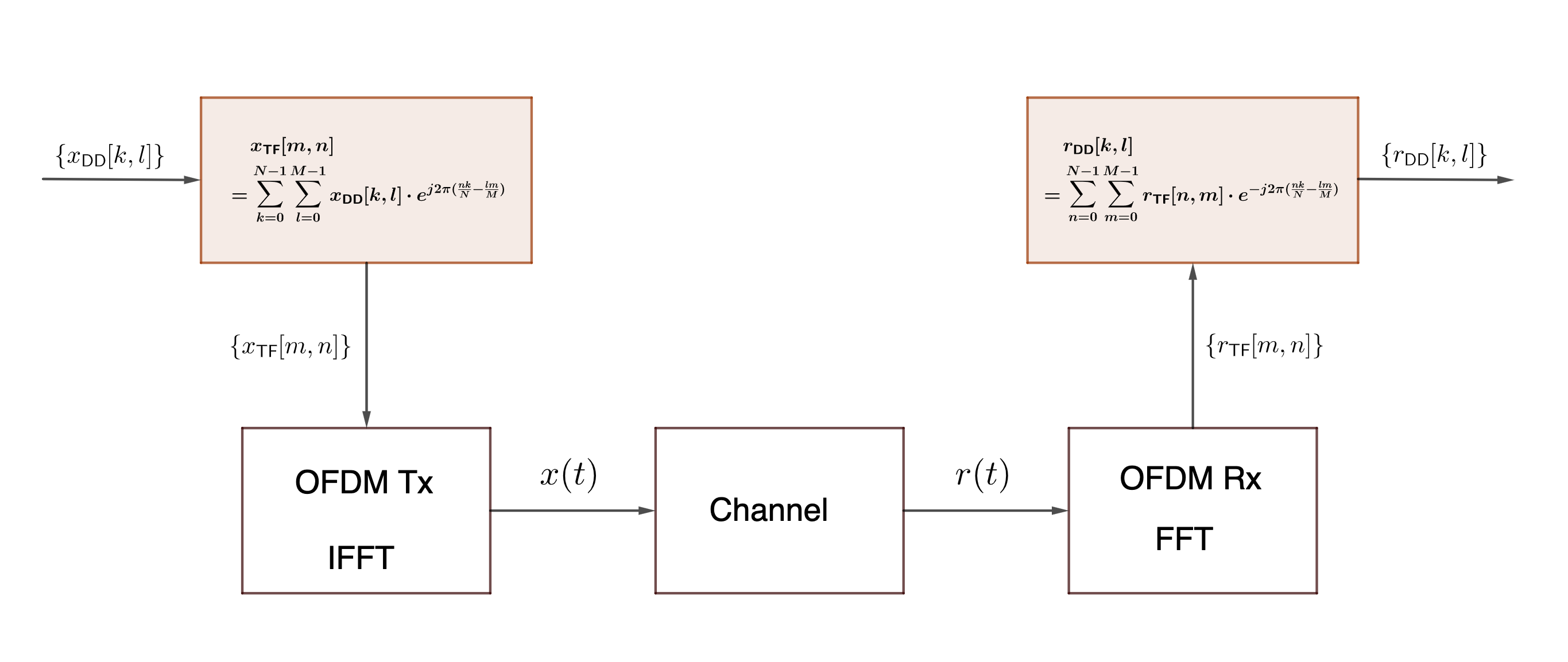 |
| OTFS Transmitter and Receiver based on OFDM |
Proof: The key is to evaluate the inner product
\[\langle \alpha_{(k,l)} , \beta_{(n,m)}\rangle = e^{j2\pi (\frac{nk}{N} - \frac{ml}{M})}\]which can now be evaluated in brute force. The literature of this derivation is quite complete, with the additional generality of allowing different symbol waveforms (one doesn’t have to use sinc function to modulate symbols.) Instead of repeating those derivations, we will give two slightly hand-waving ways to help the readers to get to the result easily. This, hopefully, reveals the gist of the issue.
First, we can do some rough computation to get the main idea.
The key is to realize that \(\alpha_{(k,l)}\) is time limited to \(N\) small intervals: \(\left[n'T + l\frac{T}{M}, n'T + (l+1)\frac{T}{M}\right]\) for \(n'=0, \ldots, N-1\), and \(\beta_{(n,m)}\) is also time limited to \([nT, (n+1)T]\). So there only a single sub-interval from the support of \(\alpha_{(k,l)}\) that overlap with \(\beta_{(n,m)}\). We can thus directly write the inner product as an interval within that interval.
\[\begin{align*} \langle \alpha_{(k,l)}, \beta_{(n,m)}\rangle &= \int_{nT + l \frac{T}{M}}^{nT + (l+1)\frac{T}{M}} \; \alpha_{(k,l)}(t) \cdot \beta_{(n,m)}^\dagger (t) \; dt\\ &= \int_{nT + l \frac{T}{M}}^{nT + (l+1)\frac{T}{M}} \; \sqrt{\frac{T}{MN}} s\left(t - l \frac{T}{M} - nT\right) \cdot e^{j2\pi \frac{kn}{N}} \cdot \mathrm{sinc}\left(\frac{t-nT}{T}\right) \cdot e^{-j2\pi m \frac{t}{T}}\; dt \end{align*}\]Now we can define \(u = t-l\frac{T}{m} - nT\), we can write
\[\begin{align*} \langle \alpha_{(k,l)}, \beta_{(n,m)}\rangle &= \int_0^{\frac{T}{M}} \sqrt{\frac{T}{MN}} \cdot s(u) \cdot \mathrm{sinc}\left(\frac{u+ l\frac{T}{M}}{ T}\right) \cdot e^{-j2\pi \frac{m}{T} u} \; du \cdot e^{j2\pi \frac{kn}{N}} \cdot e^{-j2\pi \frac{ml}{M}} \end{align*}\]The observation is that the integral is over a narrow interval of length \(T/M\). The slight changes due to \(l\) and \(m\) can both be upper and lower bounded by fixed constants. Consequently, we approximately view the integral as a constant not depending on \(k,l,m,n\), which can be normalized later. We thus have “proved”
\[\langle \alpha_{(k,l)}, \beta_{(n,m)}\rangle \propto e^{j2\pi \frac{kn}{N}} \cdot e^{-j2\pi \frac{ml}{M}}\]as desired.
Alternatively, here is a figure that helps to illustrate the idea.
In the following figure, we have two illustrations, \(\beta_{(n,m)}\) in the T-F domain on the left and \(\alpha_{(k,l)}\) in the D-D domain on the right. In both plot, the horizontal axis is time from \(0\) to \(NT\), and the vertical axis is the phase shift in radians. We use colored lines to indicate a basis function when it has a significant transmitted power. For example, this can be in the main lobe of a sinc function.
On the left, the basis function \(\beta_{(n,m)}\) is indicated by the solid blue line. It has its support on \([nT, (n+1)T]\). The phase shift is \(2\pi m \frac{t}{T}\). It starts as \(0\) at \(t= nT\), and increase linearly with \(t-nT\), with a slope determined by \(m\). Changing the value \(n\) result in shifting the entire waveform to a different interval \([n'T, (n'+1)T]\), as shown in the green dashed line. Changing \(m\) affects the slope of the phase shift w.r.t. \(t\), with an example shown in purple.
On the right, the basis function \(\alpha_{(k,l)}\) is illustrated in the same way. Here, each basis function consists of \(N\) equally spaced short intervals, each of length \(T/M\): \([nT + l \frac{T}{M}, nT + (l+1) \frac{T}{M}]\) for \(n=0, \ldots, N-1\). Because these intervals are short, we simply think the phase shift within each short interval as a constant. There is a linear increment of phase shift determined by \(k\). In the figure, \(\alpha_{(k,l)}\) is illustrated as \(N=4\) pieces of red segments, each with length \(T/M\). Changing the value of \(l\) result in a different basis with support on a non-overlapping set of short intervals, shown in green for example. Changing the \(k\) value would result in a different rate of change in the phase shift between the small intervals, as shown in the purple examle.
The key to compute the inner product between the two basis functions is to overlap the two figures. For example, the blue signal and the red signal would only overlap in the interval \([nT + l\frac{T}{M}, nT+ (l+1)\frac{T}{M}]\). This interval is so short that the pulse shape within does not matter much. The only thing important is to find out the phase difference between the two. The phase shift at the point of intersection on the blue curve is \(2\pi m \frac{t}{T}\vert_{t=l\frac{T}{M}} = 2\pi \frac{lm}{M}\). The phase shit on the red curve at the same point is \(2\pi \frac{kn}{N}\). The difference between the two phase shifts is the inner product (and conjugate).
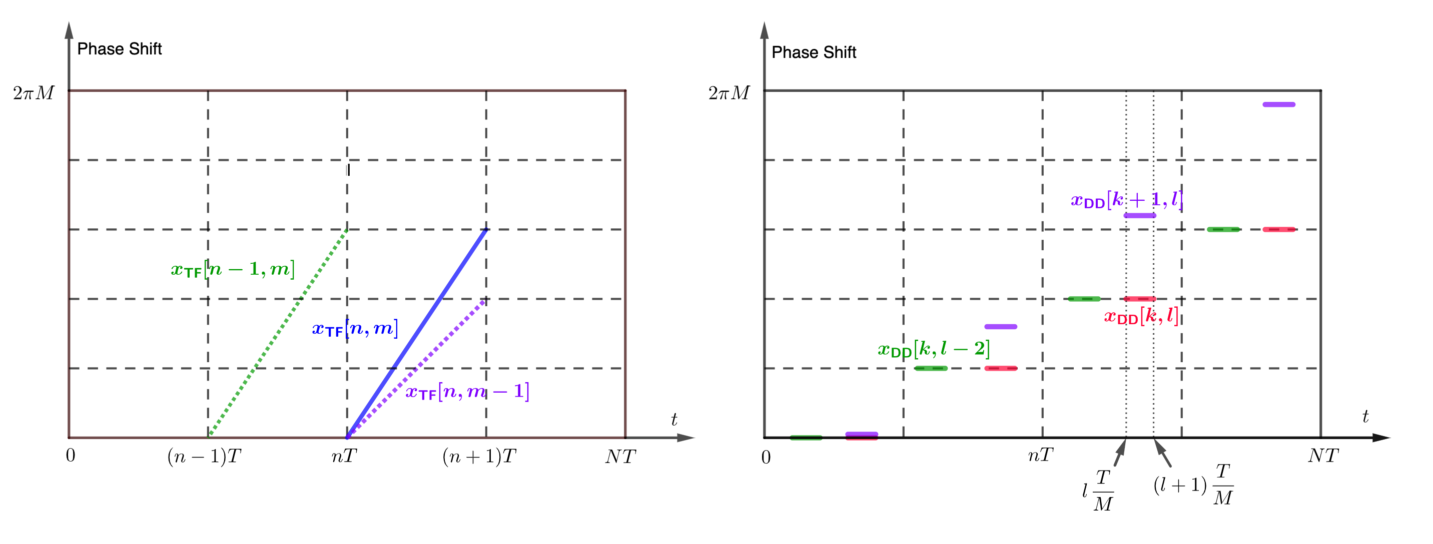 |
| Illustration of basis functions in the T-F domain (left) and the D-D domain (right). |
\(\blacktriangle\) The Sparsity in DD-Domain, a Numerical Experiment
Here is an experiment to see how the OTFS modulation allows a relatively sparse ISI pattern.
Enjoy Reading This Article?
Here are some more articles you might like to read next: